
Sparse Matrix Vector Multiplication
spMV = (sparse matrix vector multiplication and accumulation)
Dense vectors = no elements are zero vs. Sparse matrix mult = most of the elements are zero. An example is a matrix representing the coefficients in a linear system of equations. Each row is an equation, but each equation has a small number of variables.
A real use case: matrices used to solve linear systems of N equations of N variables
1st approach: A * X + Y = 0, A = N by N matrix, X = vector of N vars, Y = vector of N constant vals, solve for X to satisfy all equations
Problem: storing these elements waste memory capacity, memory bandwidth → there are methods to reduce the energy it takes, but it causes irregularity → irregularity leads to underutilization of memory bandwidth, control flow divergence, load imbalance in parallel computing
2nd approach: invert the matrix: X = A^-1 * (-Y)
Problem: size of the matrices can overwhelm this approach — Inverse sparse matrix is larger than OG → Inversion process generates many nonzero elements = fill-ins…makes it impractical
When sparse mult is positive-definite:

Meaning: the gradient of solving x for Ax=B equation is set to 0
A better approach is to use iterative algorithms, specifically the Conjugate Gradient method. The point of it is to guess so it converges to the true answer. Conjugate means orthogonal to A.
Steps: guess a solution for x → perform A * X + Y → is result close to 0 vector
- If not refine the guessed X with a gradient vector formula → another iteration of A * X + Y

initial guess for a solution vector
We want to find the rate of error (residual) and if the residual is less than a chosen tolerance, X is accepted as the solution
If the residual is not close to 0 → use residual and search history to make the next conjugate direction → performs another iteration
Doing it by iterations makes it easier means computations are not being wasted on wasted 0s or inefficient computations. Sparse matrix storage have one goal: reduce the zero elements.
Sparse matrix storage formats rely on:
- Space efficiency: the amount of memory capacity that is required to represent the matrix using the storage format
- Flexibility: the extent to which the storage format is able to add or removing nonzeros
- Accessibility: the kinds of data that the storage format makes it easy to access
- Memory access efficiency: the extent to which the storage format enables an efficient memory access pattern for a particular computation
- Load balance: the extent to which the storage format balances the load across different threads for a particular computation
Coalesced memory vs. noncoalesced:
32 threads in a warp means 32 byte memory sectors. This means 32 * 32 = 1024 bytes transferred, but only 128 bytes are actually used. 12.5% are being used which is poor efficiency. With coalesced access, 32 threads * 4 bytes = 128 bytes. 128 bytes used / 128 bytes transferred = 100% efficiency.
Control divergence = Warp divergence
- threads within the same warp execute the same instruction
- problem: if-else, switch loops make them execute on different execution paths
- impact: serialize (meaning GPUs execute instructions sequentially instead of in parallel)
Storage formats:
(1) COO = Coordinate List format
Nonzero vals are stored in a value array. Row and column arrays are taken which shows the storage overhead; Usually is less in spMv.
For sparse matrices, the majority of elements are zero → overhead < space ; saved by not storing zeroes
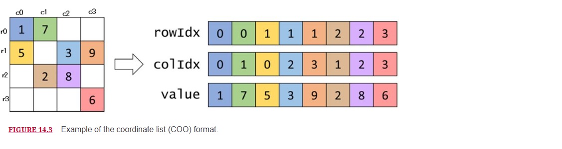 Source: Figure 14.3 – A simple SpMV kernel with the COO format
Technique: assign a thread to each nonzero element
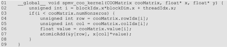 Source: Figure 14.5 – A parallel SpMV/COO kernel
- Int i = index of nonzero element
- If statement = make sure it is within bounds
- Thread identifies row, col, value array
- Float value = ( col index * nonzero val)
Atomic operations are used to accumulate because multiple threads can update the same output element
- con: no accessibility – same output is updated by multiple threads
In the COO format, we can process the elements in any order wanted. If you do not want to put the values 1, 2, 3, 4…in numerical order, you can readjust the order and their associated row and column indexes. The order the values are processed does not matter when it comes to calculating the correct final answer.
COO - memory access is coalesced because consecutive threads access consecutive elements to form the COO format
Load Balance - each thread is responsible for each nonzero element → all threads responsible for the same work → no control divergence except for at the boundary
(2) Compressed sparse row (CSR) storage format
Need to fix accessibility: avoid this making the same thread responsible for the nonzeroes in a row + parallelization across rows in spMV
Size: # of rows + 1 = 4 + 1 = 5
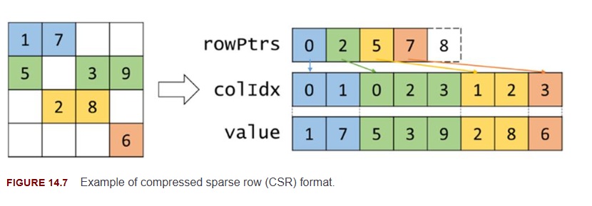 Source: Figure 14.7 Example of compressed sparse row (CSR) format - 14.3 CSR format
When we categorize the rows this way, the memory access patterns are easy to see.
rowPtr = Row Pointer Start: row 0 = r0 contains 2 elements 0 + 2 = 2 [0,2]
3 elements in r1 = 2 + 3 = 5 [0,2,5]
2 elements in r2 = 5 + 2 = 7 [0, 2, 5, 7]
1 element in r3 = 7 + 1 = 8 [0, 2, 5, 7, 8]
Max of 5 for CSR size
In CSR the row index is out, the rowPtr is viewed as the row major layout of matrix (without the zero elements). Without atomic operations, each row is traversed by a single thread, each threads writes to a distinct output val.
Space efficient: CSR is more space efficient than COO. 3 arrays needed for COO, 2 arrays needed for CSR (colIdx, value) with rowPtr only needed as many elements as Rows + 1 → size is smaller than rowIdx array in COO
Flexibility: CSR is less flexible than COO because it adds nonzeroes,
COO — nonzero can be added by appending it to the ends of the arrays
CSR — nonzero must be added to the specific row it belongs to → nonzero elements in later rows need to be shifted → row pointers of later rows have to be incremented → CSR matrix more expensive to add
Accessibility: CSR avoids atomic operations which is better at parallelization across rows. But…based on certain situations: application does not have enough rows to utilize all GPU threads, it is better to use COO format for more parallelism.
Load balancing: Causes flow divergence in warps — # of iterations a thread takes is dependent on the # of nonzero elements in rows that could be random → distribution of nonzero elements among rows can be random → adjacent rows have different # of nonzero elements → flow divergence in warps
More info at 14.2 and 14.3 of Programming Massively Parallel Processors
(3) ELL format
To address non-coalesced memory access, we can apply data padding and transposition on the sparse matrix data. The ELL storage format picks up on that. Like CSR, but adding padding elements to the other rows to make them the same length as the max length rows. Now the matrix is a rectangular. This is the same as transposing the rectangular matrix in row order (in C).
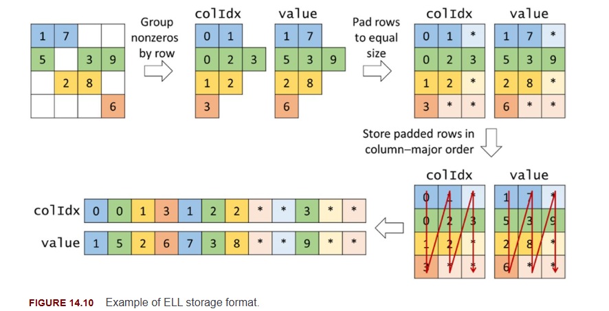 Source: 14.4 - Figure 14.11 Example of parallelizing SpMV with the ELL format.
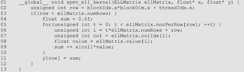 Source: 14.4 - Figure 14.12 A parallel SpMV/ELL kernel
//02 each thread is assigned to a different row of the matrix //03 boundary check ensures that the row is within bounds //05 dot produce loop goes through the nonzero elements of each row
Now: input matrix has a vector ellMatrix.nnzPerRow – writes down the # of nonzeros in each row + each thread iterates only through the nonzeros in its current row
- If input matrix does not have this vector → kernel iterates through all elements → including padding → padding = value 0 → will not affect output values
//06 matrix stored in column order, index i found by [iteration num * # of rows] + row index
//07 threads loads the column index
//08 thread loads nonzero vals from ELL matrix arrays
//coalesced because index i is in terms of row (threadIdx.x)
//09 input val * nonzero val += sum
//11 added to output vector; //04 sets sum back to 0 when reiterating
Space efficiency: ELL format adds more padding elements, more space overhead, makes it less space efficiency than CSR
Flexibility: ELL is more flexible when adding nonzeroes; CSR requires readjusting the arrays when adding. No readjusting in ELL as long as the row does not go over the max num of nonzeroes.
Accessibility: ELL beats CSR and COO. We can access (we know the index of nonzero element, row, col index of element)
- Index i of nonzero element: i = t*ellMatrix.numRows + row
- Row of nonzero element: row = i%ellMatrix.numRows
- row < ellMatrix.numRows → row%ellMatrix.numRows = row
Memory access efficiency: elements in column order meaning adjacent threads access adjacent memory location → memory coalescing → efficient memory bandwidth achieved
Load imbalance: SpMV/ELL has the same load imbalance as SpMV/CSR; each threads loops over # of nonzeroes in each row → does not address control divergence
This calls for a method to control the number of padded elements when we convert from the CSR format to the ELL format.
(4) ELL-COO format
Problems come up when a small number of rows have a large amount of nonzero elements. If we were able to “take away” some elements from the rows, the less padded elements needed, and the less control divergence.
The COO format can be used to curb the length of rows in the ELL format. Before we convert a sparse matrix to ELL we can take some of the nonzero elements and put them in a separate COO storage. The remaining elements will use SpMV/ELL. Excess elements removed mean the padded elements decrease, to finish it off we use a SpMV/COO.
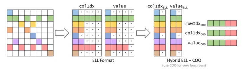 Source: 14.5 - Figure 14.13 Hybrid ELL-COO example.
Does separating the COO elements make too much overhead? Yes and no. If a sparse matrix is used in 1 SpMV calculation, then yes the extra work is overhead. If the SpMV is calculated on the same sparse kernel repeatedly and iteratively, the same matrix and their coefficients (elements) of the linear system stay the same in each iterations. The x and y vectors are different.
Space efficiency: ELL-COO has better space efficiency than ELL alone because less padding is required.
Flexibility: ELL-COO is more flexible than ELL; hybrid COO-ELL lets us add nonzeros by replacing padding elements
Accessibility: ELL is better than ELL-COO at accessing. Accessing can only be done for the rows that are in ELL format. If the rows overflow to the ones in COO, searching for them would be expensive
Memory access efficiency: SpMV/ELL and SpMV/COO have coalesced memory accesses
Load balancing: removing nonzeroes in the long rows reduces control divergence → nonzeroes in COO part aren’t affected by control divergence → no control divergence
(5) JDS Format
Can we reduce control divergence without padding? Is that only way to have coalesced memory access? JDS (Jagged diagonal storage) sorts the rows according to their length (longest to shortest).
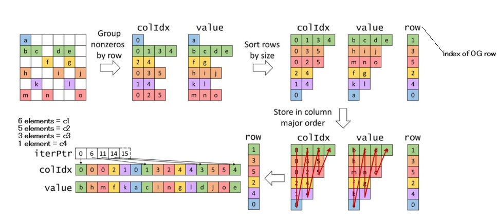 Section 14.6 - Figure 14.14 Example of JDS storage format.
Looking at Colidx each column have # of elements.
- iterPtr = 0, 6 elements in column 1 → 0 + 6 = 6
- iterPtr = 6, 5 elements in column 2 → 6 + 5 = 11
- iterPtr = 11, 3 elements in column 3 → 11 + 3 = 14
- iterPtr = 14, 1 element in column 4 → 14 + 1 = 15
Iterarr array shows where the nonzeroes of each iteration begin → coalesced memory
JDS version 2: the rows can be put into sections of rows after being sorted → ELL representation for each section → pad the rows to match max length row → reduce padding comparing to ELL → iterPtr not needed here → need a section pointer array that points to the beginning of the ELL section
As long as the y elements are adjusted if the rows are readjusted, you can reorder the equations which gives us the correct solution to linear equations. One final step would be to reorder the final solution back to the OG using the row array. Using an iterative solver makes overhead not a problem.
Space efficiency: JDS avoids padding…better than ELL. The JDS variant with padding has less padding that the ELL format.
Flexibility: JDS is not flexible to add nonzereos — changes the sizes of rows which means rows have to be resorted
Accessibility: JDS can access given a row index and nonzero elements in that row, but not easy to access if given a nonzero, row index, column index of a nonzero
Memory access efficiency: JDS stores nonzeroes in column order → coalesced manner → no padding required → starting locations of each memory access/iteration is allowed to vary → no iterations can start specific alignment boundaries → cannot force memory access start points to align → JDS less efficient that ELL
Load balance: JDS sorts rows of the matrix so that threads in the same warp iterate over rows of similar length → reduces control divergence
Pop quiz time! These are exercises from Chapter 14.
- Represent the matrix each of the following formats: (1) COO, (2) CSR, (3) ELL, and (4) JDS.

(1) COO– has a row, col index, value array
Row idx = [0,0,1, 2, 2, 3, 3]
Col idx = [0, 2, 2, 1, 2, 0, 3]
Value array = [1, 7, 8, 4, 3, 2, 1] left to right nonzero values
- CSR–has rowPtr, col index, value array
RowPtr = [0, 2, 3, 5, ,7]
Col idx = [0, 2, 2, 1, 2, 0, 3]
Valarray = [1, 7, 8, 4, 3, 2, 1]
rowPtr: current ptr + num of elements in row
0 + 2 = 2
2 + 1 = 3
3 + 2 = 5
5 + 2 = 7
Rows + 1 = 4 + 1 = 5 size for CSR rowPtr array
The rest of the answers are in this repo: https://github.com/tugot17/pmpp/blob/main/chapter-14/README.md
Source: Programming Massively Parallel Processors: A Hands-on Approach by Wen-mei W. Hwu, David B. Kirk, and Izzat El Hajj