
Before Profiling
2 questions to answer before profiling:
(1) What is the theoretical arithmetic intensity of my algorithm?
Arithmetic intensity — how many FLOPS do I need? May run multiple warps and reach a point where CPU is fully full
FLOPS = floating-point operations per second = how many computations can i run in a second
FLOP = 2 * M * K * N
Total number of calculations needed for a matrix multiplication between a M * K matrix and K * N matrix
Bytes = (MK + KN + M*N) * 4 = min number of bytes to transfer to and from global memory
MK and KN = size of the first and second input matrix
M*N = size of output matrix; each element is a float
Intensity equation: FLOP / bytes = (2 * M * K * N) / [ (MK + KN + M*N) * 4 ]
During prefill phase — takes in input as a whole (usually compute bound), answers how many computations can be made
When we say compute or memory bound, in x-bound the x is the bottleneck. Compute bound means the math units are running at max capacity and the time is limited by how fast the GPU can perform calculations. Memory bound means the memory bus (cache/RAM/VRAM transfer bandwidth) is at max capacity and the time is limited by how fast bytes can travel to compute cores. The cores then spend idle cycles waiting for data.
(2) Should my algorithm be compute-bound or memory-bound?
Decode phase — model gives answer > does it one token at time (usually memory bound) > to decide compare which is more: intensity or ridge point
BW = bandwidth = how much bandwidth needed to transfer data
Ridge = max data i can take from CPU and computations from GPU > hits peak > maxed CPU limit / how much memory i can pull or process
Ridge point = Peak FLOPS / Peak bandwidth
algorithm’s intensity > ridge point ∴ compute-bound
algorithm’s intensity < ridge point ∴ memory-bound
To also help you decide you can plot a Roofline model, plots the peak FLOPs/s (throughput — the y-axis) against the arithmetic intensity of that algorithm (the x-axis).
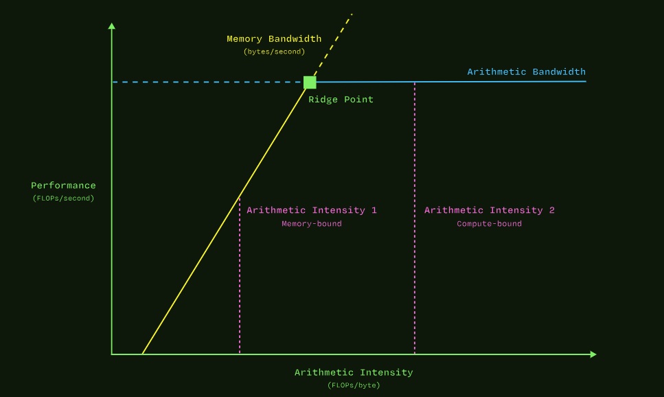
Source: modal – https://modal.com/gpu-glossary/perf/roofline-model
Left: Lower intensity → bandwidth (BW) bound & limited by the peak memory bandwidth
Right: Algorithm to the right will fully use our FLOPs
Improve an algorithm performance → increasing its arithmetic intensity → OR → increasing the memory bandwidth available
Another way to look at it is the matmul: matrix multiplication equation X * Y = Z (* is multiplying)
2 matrices using bfloat16: X has shape [B, D], Y has shape [D, F], Z has shape [B, F]
B = batch size, D and F are hidden dimensions, bfloat16 uses 2 bytes/element
X: B * D elements * 2 bytes = 2BD bytes
Y: D * F elements * 2 bytes = 2DF bytes
Z: B * F elements * 2 bytes = 2BF bytes

In LLMs the batch size B is small compared to hidden dimensions D and F → DF (size of the weight matrix) is larger than BD or BF → BD + DF + BF ≈ DF

arithmetic intensity is approximately equal to the batch size B

B < 240 kernel is memory-bandwidth bound B > 240 kernel is compute-bound
In the roofline model shown, once we hit the ridge point at 240 arithmetic intensity, the kernel will switch from memory to compute bound.
Kernel can show different metrics:
memory-bound bottleneck:
- DRAM utilization > 80% of peak — close to theoretical max
- GMEM ratio < 0.5 (operations per global memory access)
- GMEM = compute-to-global-memory-access ratio
compute-bound bottleneck:
- High FLOP counts
- Low memory pressure
- SM utilization near 100%
occupancy-limited bottleneck:
- Occupancy < 50%
- Active warps per cycle much < theoretical maximum
- Register or shared memory usage is limiting occupancy
branch divergence bottleneck:
- threads in warp take different execution paths → serialization
Multi-dimensional arrays in memory are flattened into byte layouts (tensor weights), but this bad because GPUs work in parallelism. When serialized the hardware stops working in parallel, instead sequentially, which takes away a GPU’s speed and leaves cores idle.
- branch efficiency < 100
- higher execution time that normal
GPU Memory Architecture
(1) Registers: Fastest storage with limited quantity, per-thread (2) Shared Memory: Fast on-chip memory shared among threads in a block (3) Global Memory: Main GPU memory with high bandwidth but higher latency (4) Constant Memory: Cached memory for read-only data (5) Texture Memory: Cached memory optimized for spatial locality
Profiling
Profiling is the process of analyzing how an application executes on GPU hardware to identify bottlenecks and where resources will be inefficient/not practical. It answers the question: How much memory and computational ability can the hardware take right now? GPUs can do complex math, but even they have limits on the chip. Profiling identifies where the GPU is idling and how close you are to that limit.
Some profile tools are specific to looking at different parts of GPUs. NVIDIA Nsight Systems (nsys) specifically look into timeline tracing (CPU-GPU interaction, API calls, memory copies). NVIDIA Nsight Compute (ncu) looks into instruction-level counters and Roofline analysis.
Profiling measures metrics from the hardware counters (SM, PCIe interfaces, etc.) on a chip based on these 4 areas:
-
Kernel execution time + Timeline tracing: when tasks run across CPU threads, CUDA streams, GPU engines — shows where synchronizing threads are being stalled, idle GPU time between tasks
-
Compute vs. Memory Bound: is execution being blocked by floating-point math throughput (Tensor cores) or memory bandwidth (hitting caches/VRAM) — tool to use to see this is Roofline Model
-
Memory Access Efficiency:
- Memory Coalescing: Are threads in a warp using continuous memory addresses or fragmented/serialized memory requests?
- Cache Hit Rates: Hit/miss ratios for L1/Shared Memory and L2 cache
- PCIe / Interconnect Transfers: Time spent copying data between host RAM and GPU VRAM
- Warp Scheduling & Occupancy:
- Theoretical vs. Achieved Occupancy: active warps per SM divided by hardware limit (often restricted by register usage or shared memory size)
- Warp Divergence: How often threads in a warp take different branches (ex. if/else statements) → forcing the GPU to serialize execution paths
- Stall Reasons: Specific hardware causes keeping warps from executing (ex. synchronization barriers, math pipe throttles, etc.)
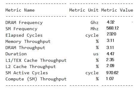
Analysis: This kernel grid is too small to fill the available resources on this device, resulting in only 0.2 full waves across all SMs. Look at Launch Statistics for more details.
…

Est. Local Speedup: 74.62%
The difference between calculated theoretical (50.0%) and measured achieved occupancy (10.8%) can be the result of warp scheduling overheads or workload imbalances during the kernel execution.
Load imbalances can occur between warps within a block as well as across blocks of the same kernel.
--------------------------------------------------------------------------------------------------------------
Est. Local Speedup: 50%
The 4.00 theoretical warps per scheduler this kernel can issue according to its occupancy are below the hardware maximum of 8.
This kernel's theoretical occupancy (50.0%) is limited by the number of blocks that can fit on the SM, and the required amount of shared memory.
--------------------------------------------------------------------------------------------------------------
Est. Speedup: 8.57%
One or more SMSPs have a much lower number of active cycles than the average number of active cycles.
Maximum instance value is 27.12% above the average, while the minimum instance value is 100.00% below the average.
Profiler steps
1. Identify which kernel or data transfer steps consume the bulk of execution time
ncu --kernel-name "mykernel" --launch-skip 5 --launch-count 1 \
    --set full -o baseline ./myapp
mykernel = specify kernels matching name
–launch-skip 5 = skips first 5 launches of mykernel; avoid cold start effects (initial memory allocations…) to get profile steady-state execution
–launch-count 1 = profiles 1 launch of the kernel after skipping first 5 → stops profiler → prevents profiler from hanging if kernel runs in a long loop
–set full = collects hardware metrics (Roofline model, warp state stats)
-o baseline = saves report to baseline.ncu-rep = file in Nsight compute GUI
./myapp = executable to launch/monitor
Metrics collected are:
- Kernel Execution Time: Total time spent executing the kernel, Grid Size: # of blocks launched, Block Size: # of threads per block, Active Warps: Average number of active warps per SM
- DRAM Throughput: Data transfer rate between GPU and memory, L2 Cache Hit Rate: % of L2 cache hits, Shared Memory Bank Conflicts: # of bank conflicts causing serialization
- Occupancy: Ratio of active warps to maximum possible warps, Warp Execution Efficiency: % of active threads in warps, Branch Divergence: Impact of divergent branches on performance (too many branches lower performance)
2. Identify the limiting subsystem
This means a user should look at the kernel metrics to identify the bottleneck:
(1) Compute bound — Go to Compute Workload Analysis section on the Details page
- Look at the pipelines, the one with the highest % is the bottleneck (2) Memory bound — Go to Memory Workload Analysis section on the Details page
- Memory Chart shows data flows between DRAM, L2, L1, and SM with bytes and % of Peak
Ex.
Peak DRAM > 75% ∴ kernel uses bandwidth well
Peak DRAM < 50% ∴ waste (non-coalesced accesses, excessive L2 traffic, etc.)
Internal congestion — Go to Memory Workload Analysis section, Shared Memory and L1/Cache tables
Look for:
-
Memory > 60%, DRAM < 30%
-
Ratio of shared memory requests compared to global memory requests
- Ratio < 5 ∴ poor reuse
- Normal: 5–20
- Ratio > 20 ∴ low DRAM + kernel spends more time LDS/STS instructions rather than DDMA + LSU pipeline has too much internal traffic
- FMA vs total instructions ration — Instruction Statistics section on the Details page
- ratio < 30% in a compute-intensive (GEMM) kernel ∴ compute units starved by internal memory instruction
Latency bound — Scheduler Statistics and Warp State Statistics
Look for:
- Scheduler Statistics section — No Eligible (% of cycles where no warp is ready) > 30% ∴ scheduler is waiting for majority of time + Eligible Warps per active cycle < 1 ∴ need more warps to hide latency
- Scheduler Statistics section — Issue Slot Utilization rule: how many warps are active vs eligible; ex. Every scheduler is capable of issuing one instruction per cycle, but for this kernel each scheduler only issues an instruction every 5.4 cycles
- Warp State Statistics section — dominant stall reason in the bar chart to look at is Not-issued: stalls that reduce throughput because no eligible warp could be scheduled
3. Identify what is being wasted and how to estimate the speedup
Amdahl’s Law
GPUs use the same instruction on multiple threads (parallel execution). Some tasks can be be parallelized and run on the GPU, others need to be run on the CPU. When we use multiple processors, how much faster does a task take? That is defined by Amdahl’s Law.
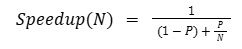
P = Fraction of the amount of tasks that can be parallelized (0 ≤ P ≤ 1)
N = Number of processors
Ex. 60% of tasks are parallelizable (P = 0.6), using 2 processor

How let’s play with the numbers a bit.

After profiling and finding the inefficient parts, we can optimize. Profiling starts at the system level, but optimizing becomes silly if the GPU spends time waiting for data from the CPU.
Problems
Problem 1) Non-Coalesced Global Accesses
Coalescing is when threads in a warp access shared memory locations, multiple memory requests make for fewer transactions.
Good vs. bad example
__global__ void coalesced_access(float *data, int n) {
int thrid = blockIdx.x * blockDim.x + threadIdx.x; //thread index that defines a segment of data in a block
if (thrid < n) { //out-of-bounds check
//data[thrid] = data[thrid] * 2.0f; // GOOD: consecutive threads access consecutive addresses
//data[tid * stride] = data[tid * stride] * 2.0f; // BAD: Strided access pattern
 }
}
Look at the Memory Workload Analysis section for the Sectors per Request column. (BW = Bandwidth)
BW waste = (Sectors/Req — 4) / (Sectors/Req)
Potential speedup (if DRAM-bound) = (Sectors/Req) / 4
Ex.: Sectors/Req = 16
Waste = (16–4) / 16 = 75%
Potential speedup = (16 / 4) = 4x ∴ too big
Ex. Sectors/Req = 5
Waste = (5–4) / 5 = 20%
Potential speedup = (5 / 4) = 1.25x ∴ better but not great
If the kernel is not DRAM-bound, the actual speedup will be less than the potential because the bottleneck is somewhere else.
Problem 2) Excessive Global Traffic Volume
Look at the Details page: shows Sectors/Req = 4 (coalescing OK) but the total number of bytes transferred can be excessive → to check look at dram__bytes.sum in the Memory Workload Analysis section
Traffic overhead = dram__bytes.sum / theoretical_bytes
Traffic overhead > 2 ∴ kernel re-reads data that should be reused
Problem 3) Shared Memory Bank Conflicts
if the kernel spends a fraction f of its time on shared loads → bank conflicts multiply that time by n
Bank conflicts are when multiple threads within the same warp try to access different memory addresses that are in the same physical memory bank of shared memory. The hardware cannot answer the requests in parallel, meaning the requests are then done sequentially with increased latency.
Speedup = 1 / [(1 — f) + f/n]
Ex. 60% time on shared loads, conflicts are 3-way (each load takes 3 passes) → conflicts are eliminated → shared time drops to 0.2 with a speedup of 1 / [(1–0.6) + 0.6/3] = 1 / 0.6 = 1.67x.
Shared memory is critical for optimizing GPU kernels. Faster access than global memory.
Conflicts occur when:
- GPUs have 32 shared memory banks
- Accessing different addresses in the same bank serializes the access (flat, no parallel execution)
- Adding padding (ex. [TILE_SIZE+1]) can prevent conflicts
Solutions:
(1) Memory Padding to Prevent Bank Conflicts
__shared__ float sdata[32][32]; // 32 columns = 32 banks // without padding
__shared__ float sdata[32][33]; // Extra column //with padding //prevents bank conflicts
(2) Tiled Access Patterns
Let’s say we make a kernel function that takes in global VRAM and breaks it into small 16 by 16 chunks/tiles
#define TILE_WIDTH 16
…
int tx = threadIdx.x; //local coordinates within block //range: 0 - 15
int ty = threadIdx.y; //local coordinates within block //range: 0 - 15
int x = blockIdx.x * TILE_WIDTH + tx; //block’s starting col + col index
int y = blockIdx.y * TILE_WIDTH + ty; //block’s starting row + row index //tiles now created
tile[ty][tx] = input[y * width + x]; // transferring 16 by 16 tile into a 2D slice from global memory space (y * width + x) into a localized, fast on-chip 2D structure (tile[ty][tx])
Problem 4) LSU Pipeline Saturation
Bank conflicts are low (YAY) + shared/global ratio is high + FMA/total ratio is low = raw volume of memory instructions is not displayed by tools — must calculate
Memory instructions per FFMA = (LDS + STS + LDG + STG) / FFMA
Need thread coarsening the ratio is closer to 1. Each memory instruction takes a scheduler slot instead of an FFMA.
Problem 5) Insufficient Latency Hiding
The volume of traffic is fine, the time spent waiting for data is the issue.
Typical latency by access type:
HBM = 200–500 cycles
L2 = 100–200 cycles
Shared = 20–30 cycles
Register = 4–6 cycles (FMA/ALU)
Stalls have many global addrs & occupancy is low → solution: increase occupancy
Problem 6) Warp Divergence
Details page — Warp State Statistics section: If there’s a significant difference between Avg. Executed instructions and avg. issued instruction → cause: serialization (divergence or bank conflicts)
Waste calculation:
Divergence waste = 1 — (Avg Predicated-On Threads / 32)
Inactive threads still generate the memory transfer with useless data now.
Problem 7) Register Spilling
Launch Statistics section on the Details page — shows the # of registers per thread
In Nsight Compute look for STL and LDL instructions in the Source view.
spill store + spill load pair adds ~ 40–100 cycles
If the spilling is in the inner loop (instructions executed on STL/LDL), the impact is multiplied by the number of iterations vs. the spilling being in the prologue (Instructions Executed = W), the impact is generally negligible
Credit to:
- https://modal.com/gpu-glossary/readme
- Programming Massively Parallel Processors chapter. 6: Performance Considerations — David B. Kirk, Wen-Mei W. Hwu, and Izzat El Hajj
- https://www.youtube.com/@pmpp-book/videos
- https://docs.nvidia.com/cuda/cuda-programming-guide/02-basics/intro-to-cuda-cpp.html